Part 1: Fit a Neural Field to a 2D Image
This part aims to reconstruct a 2D image using a Neural Field, a simplification of the NeRF. I began by creating a Multilayer Perceptron (MLP) network with Sinusoidal Positional Encoding (PE) in PyTorch. The end goal is to input a coordinate to the model and have it output the color at that pixel. The PE increases the dimensionality of the input dimensions by applying a series of sinusoidal functions. The PE is controlled using a hyperparameter (L) that defines the frequency level at which to encode the input: as L increases, the PE encodes more complex information about the input coordinate and vice versa. The PE model used is shown below:
For my MLP, I used the model provided in the project specifications. The input layer (the size of this layer corresponds to the dimension of the encoded input determined by L) is the input coordinate encoded using the PE. This feeds into the two subsequent hidden layers (fully connected linear layers of size 256 with ReLU non-linearities). Lastly, the output layer maps the hidden features to 3 output dimensions representing RGB. A Sigmoid activation is then applied to constrain the output between 0 and 1 (valid RGB range).
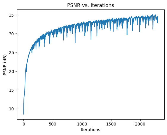
Since training the network with every pixel at each iteration is not feasible due to GPU limits, I implemented a Dataloader. The dataloader randomly samples N pixels from the image to provide the MLP for each iteration of training, where N is the batch size. Provides the MLP with data during the training process. Specifically, passing these N randomly sampled pixel coordinates along with their RGB values to the MLP allows us to supervise the training. I used mean squared error (MSE) loss between the predicted RGB and ground-truth RGB along with the Adam optimizer to train the model. However, I used the Peak signal-to-noise ratio (PSNR) computed from the MSE, as shown below, to measure the reconstruction quality of the model's predictions.
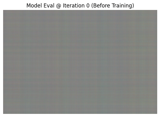
To begin, I first used the default parameters provided by the project:
- L = 10
- hidden_dimensions = 256
- batch_size = 10,000
- num_iterations = 2,300
- learning_rate = 1e-2


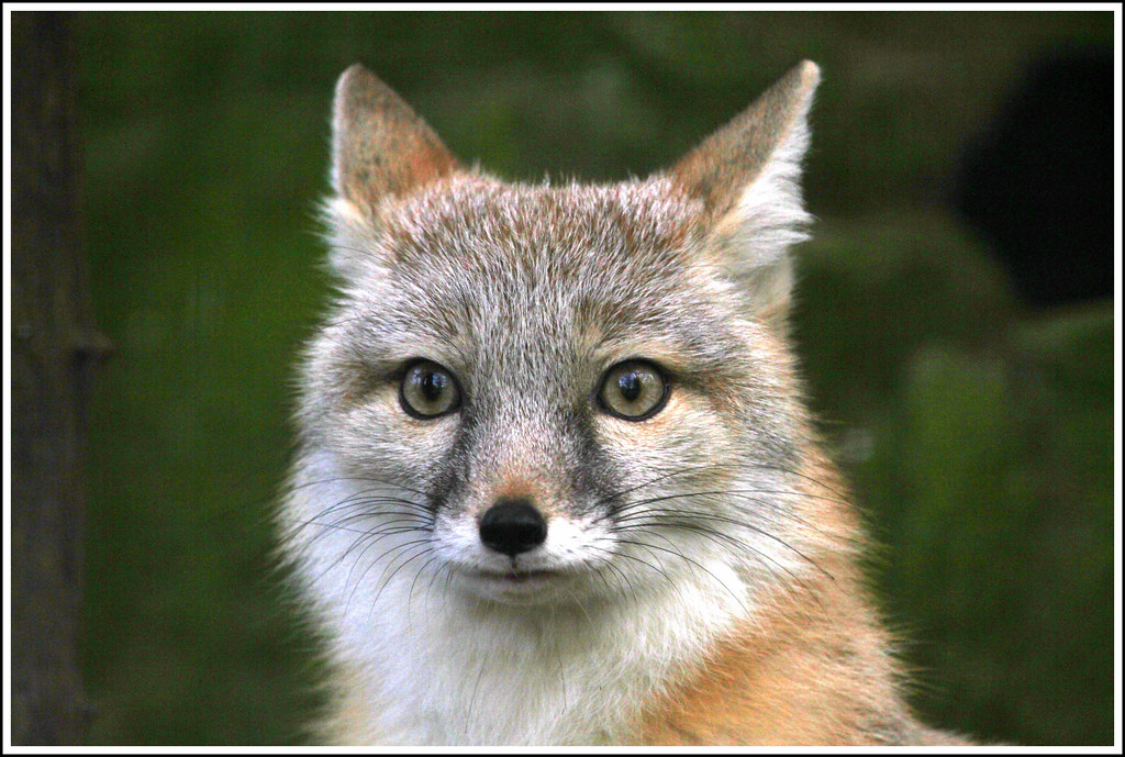
Original Image
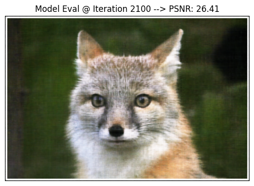
As you can see, the default hyperparameters did decently well in reconstructing the image with a final PSNR of 26.36.
Next, I aimed to fine-tune some of the hyperparameters to get a better PSNR score; specifically, I studied the effects of altering L and Learning Rate.
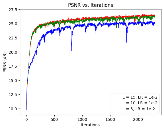
In my study of L, I kept all the other hyperparameters constant. Below are the three sets of hyperparameters that I used in this study. Note that Set 2 is identical to the default parameters–– hence, it was not trained again. Also, the input dimensions used to instantiate the model differed based on the value of L (which I've recorded below).
Set 1 Parameters:
- L = 5 (input dimension = 22)
- hidden_dimensions = 256
- batch_size = 10,000
- num_iterations = 2,300
- learning_rate = 1e-2
Set 2 Parameters:
- L = 10 (input dimension = 42)
- hidden_dimensions = 256
- batch_size = 10,000
- num_iterations = 2,300
- learning_rate = 1e-2
Set 3 Parameters:
- L = 15 (input dimension = 62)
- hidden_dimensions = 256
- batch_size = 10,000
- num_iterations = 2,300
- learning_rate = 1e-2
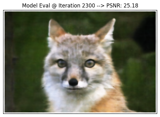
Here is how Set 1 (L = 5) performed:

Original Image
Here is how Set 3 (L = 15) performed:


Original Image
As shown in the plot below, Set 3 performed the best with a PSNR of 26.62.
From the experiments above, I concluded that L = 15 was the most ideal value of those tested. I then held L = 15 constant and studied the Learning Rate using the 3 Sets below. Note that Set 2 below was the same as Set 3 in the prior experiment–– hence, it was not trained again.
Set 1 Parameters:
- L = 15
- hidden_dimensions = 256
- batch_size = 10,000
- num_iterations = 2,300
- learning_rate = 5e-3
Set 2 Parameters:
- L = 15
- hidden_dimensions = 256
- batch_size = 10,000
- num_iterations = 2,300
- learning_rate = 1e-2
Set 3 Parameters:
- L = 15
- hidden_dimensions = 256
- batch_size = 10,000
- num_iterations = 2,300
- learning_rate = 1.5e-2
Here is how Set 1 (Learning Rate = 5e-3) performed:

Original Image
Here is how Set 3 (Learning Rate = 1.5e-2) performed:

Original Image
As you can see from the plot below, Set 2 performed the best with a PSNR of 26.62.
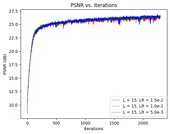
From the experiments above, I concluded that Learning Rate = 1e-2 was the ideal value for those tested. The finalized hyperparameters after tuning were:
- L = 15
- hidden_dimensions = 256
- batch_size = 10,000
- num_iterations = 2,300
- learning_rate = 1e-2
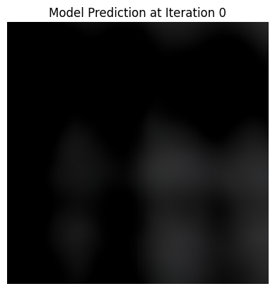
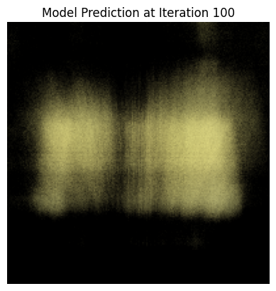
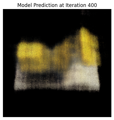
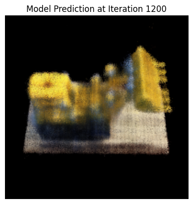
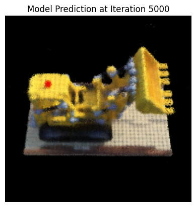
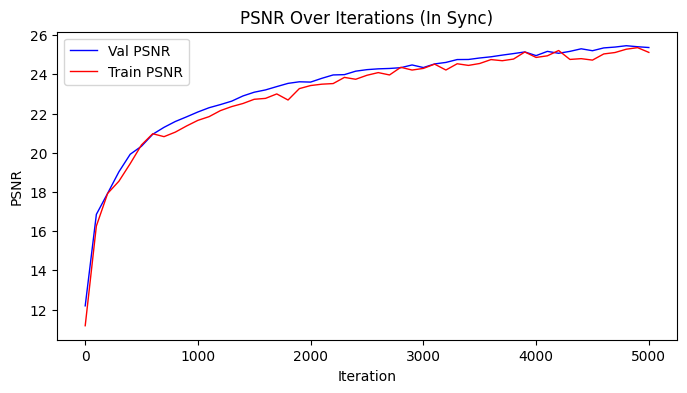
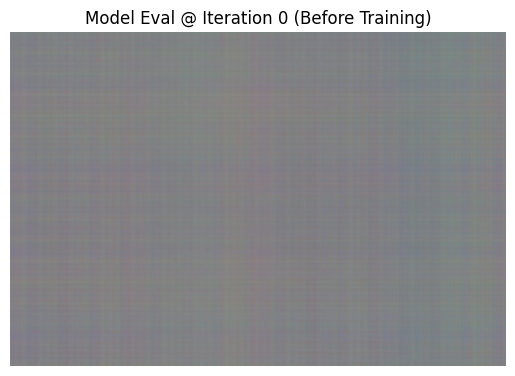
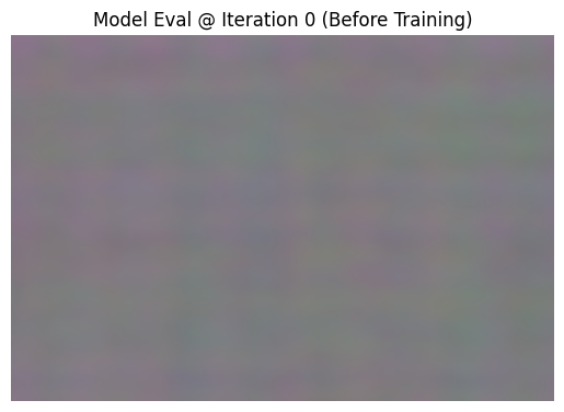
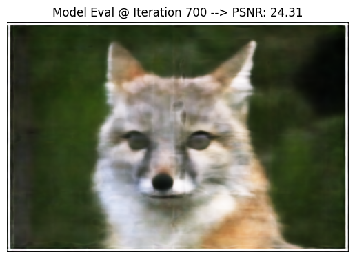
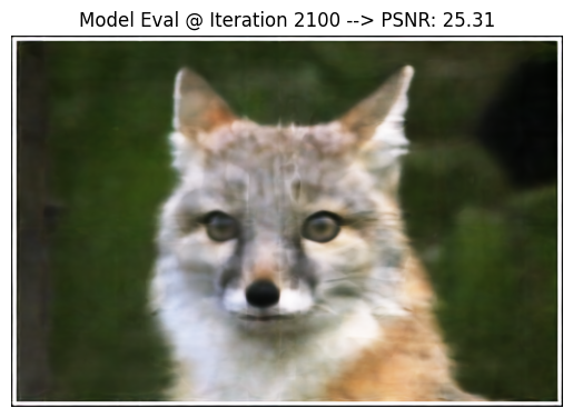
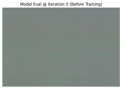
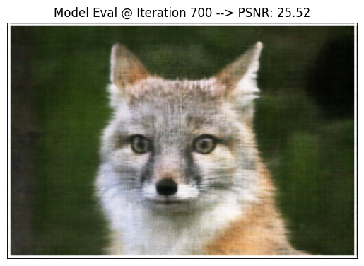
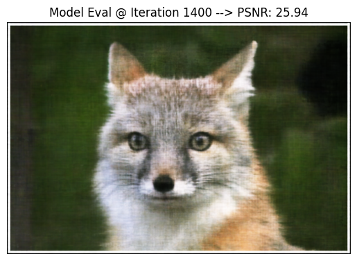
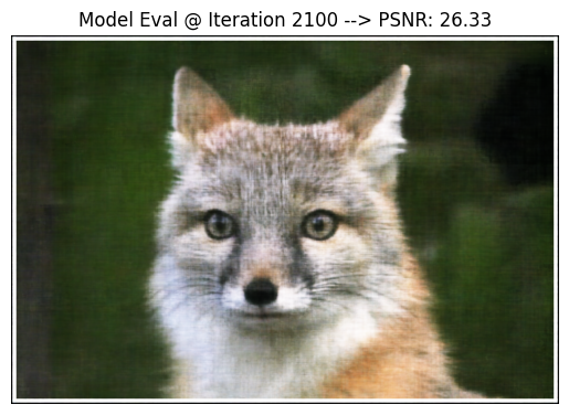
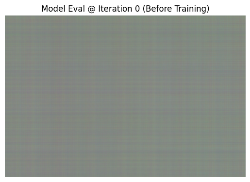
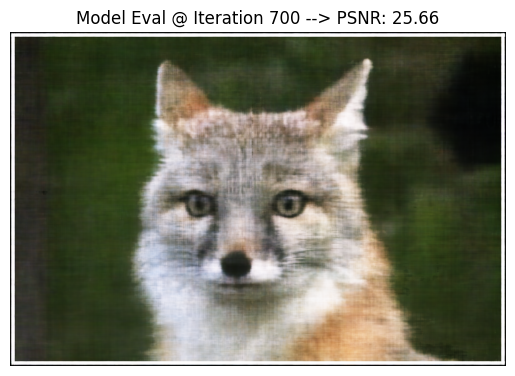
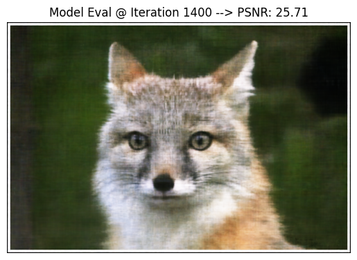
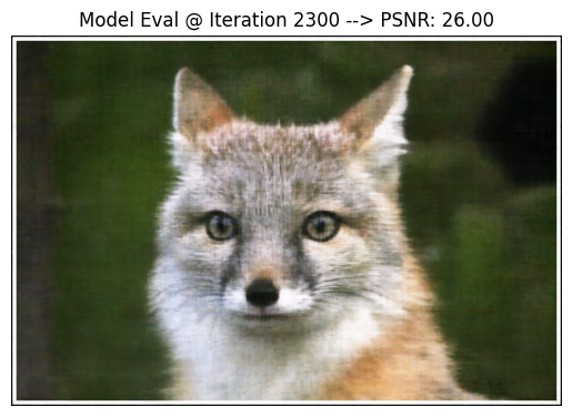
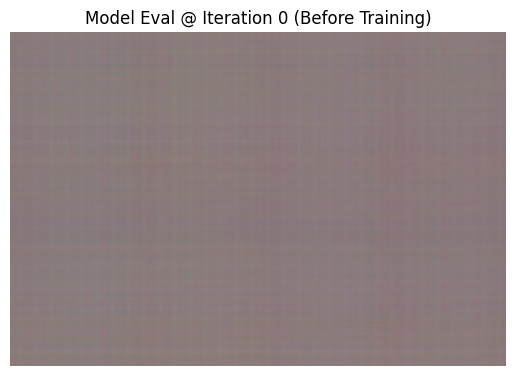
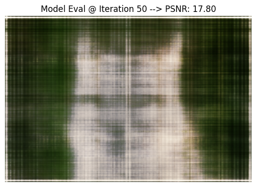
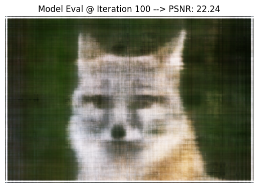
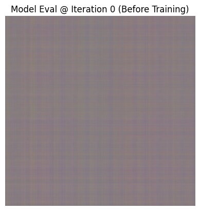
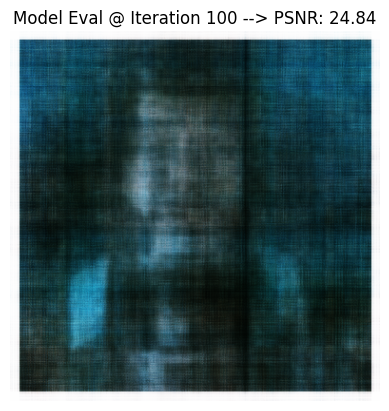
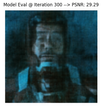
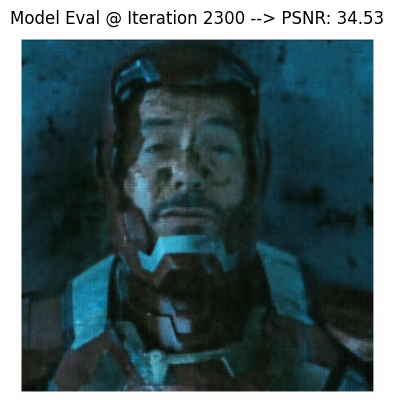
Below, I've shown the progression of training a model with these hyperparameters at strategically chosen iterations instead of the previously evenly spaced displays. I used the PSNR plot to discern iterations where noticeable changes can be seen.

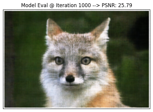

I repeated this procedure for one of my images using these finalized hyperparameters.


Original Image